Comparing different Quantities of Interest (QOIs) in ShaRP

This example demonstrates how to use ShaRP with different QOIs to analyze and explain ranking outcomes.

In this example, we will: - Set up and define two QOIs, rank and score. - Compare feature contributions under each QOI for several examples.

import pandas as pd
import numpy as np
import matplotlib.pyplot as plt
from sklearn.utils import check_random_state
import certifi
import ssl
import urllib.request

from sharp import ShaRP
from sharp.utils import scores_to_ordering


# Set up some envrionment variables
RNG_SEED = 42
N_SAMPLES = 50
rng = check_random_state(RNG_SEED)

We will use CS Rankings dataset, which contains data for 189 Computer Science departments in the US, e.g., publication count of the faculty across 4 research areas: AI, Systems, Theory, and Inter- disciplinary.

CS_RANKS_URL = "https://zenodo.org/records/11234896/files/csrankings_raw.csv"
context = ssl.create_default_context(cafile=certifi.where())

csrank_data = (
    pd.read_csv(urllib.request.urlopen(CS_RANKS_URL, context=context))
    .drop(columns="Unnamed: 0")
    .rename(columns={"Count": "Rank"})
    .set_index("Institution")
)


# Let's also preprocess this data
def preprocess_csrank_data(df):
    X = df.drop(columns=["Rank", "Score"])
    X = X.iloc[:, X.columns.str.contains("Count")]
    X = X / X.max()
    ranks = df.Rank
    scores = df.Score
    return X, ranks, scores


X, _, _ = preprocess_csrank_data(csrank_data)
X.head()


# Here we will define the scoring function
def csrank_score(X):
    weights = np.array([5, 12, 3, 7])

    # multiplier contains the maximum values in the original dataset
    multiplier = np.array([71.4, 12.6, 21.1, 13.8])

    if np.array(X).ndim == 1:
        X = np.array(X).reshape(1, -1)

    return np.clip(
        (np.array(X) * multiplier) ** weights + 1, a_min=1, a_max=np.inf
    ).prod(axis=1) ** (1 / weights.sum())


score = csrank_score(X)
rank = scores_to_ordering(score)

Next, we will configure ShaRP with qoi parameter set to rank and rank_score:

xai_rank = ShaRP(
    qoi="rank",
    target_function=csrank_score,
    measure="shapley",
    sample_size=None,
    replace=False,
    random_state=RNG_SEED,
    n_jobs=-1,
)
xai_rank.fit(X)

xai_score = ShaRP(
    qoi="rank_score",
    target_function=csrank_score,
    measure="shapley",
    sample_size=None,
    replace=False,
    random_state=RNG_SEED,
    n_jobs=-1,
)
xai_score.fit(X)

Let’s take a look at some contributions for both QOIs

contributions_rank = xai_rank.all(X)
print(contributions_rank[:5])

contributions_score = xai_score.all(X)
print(contributions_score[:5])

[[24.19268078 33.64065256 13.31261023 22.89638448]
 [23.15696649 37.52380952 13.00440917 19.35714286]
 [22.54100529 34.02425044 11.87257496 23.60449735]
 [21.57142857 33.88800705 14.43209877 21.15079365]
 [22.63932981 33.02204586 10.06084656 24.32010582]]
[[3.9695397  5.7565809  2.0867898  3.82884096]
 [2.82709753 5.00137085 1.53866678 2.14089767]
 [2.08894519 3.64974124 1.0434509  2.40865841]
 [1.88178467 3.40059394 1.30160139 1.93270165]
 [1.81081692 3.04055479 0.71759102 2.19567226]]

Now let’s plot the waterfall plots for different universities and check if the results for score and rank differ

# Plot for Stanford University, ranked #6 in QS World University Rankings 2025
plt.figure(figsize=(10, 6))

plt.subplot(1, 2, 1)
xai_rank.plot.waterfall(
    contributions=contributions_rank[5],
    feature_values=X.iloc[5].to_numpy(),
    mean_target_value=rank.mean(),
)
plt.title("Stanford University - Waterfall Plot for Rank")

plt.subplot(1, 2, 2)
xai_score.plot.waterfall(
    contributions=contributions_score[5],
    feature_values=X.iloc[5].to_numpy(),
    mean_target_value=score.mean(),
)
plt.title("Stanford University - Waterfall Plot for Score")

plt.tight_layout()
plt.show()


# Plot for University of Texas at Austin, ranked #66 in QS World University Rankings 2025
plt.figure(figsize=(10, 6))

plt.subplot(1, 2, 1)
xai_rank.plot.waterfall(
    contributions=contributions_rank[15],
    feature_values=X.iloc[15].to_numpy(),
    mean_target_value=rank.mean(),
)
plt.title("University of Texas at Austin - Waterfall Plot for Rank")

plt.subplot(1, 2, 2)
xai_score.plot.waterfall(
    contributions=contributions_score[15],
    feature_values=X.iloc[15].to_numpy(),
    mean_target_value=score.mean(),
)
plt.title("University of Texas at Austin - Waterfall Plot for Score")

plt.tight_layout()
plt.show()


# Plot for Indiana University, ranked #355 in QS World University Rankings 2025
plt.figure(figsize=(10, 6))

plt.subplot(1, 2, 1)
xai_rank.plot.waterfall(
    contributions=contributions_rank[53],
    feature_values=X.iloc[53].to_numpy(),
    mean_target_value=rank.mean(),
)
plt.title("Indiana University - Waterfall Plot for Rank")

plt.subplot(1, 2, 2)
xai_score.plot.waterfall(
    contributions=contributions_score[53],
    feature_values=X.iloc[53].to_numpy(),
    mean_target_value=score.mean(),
)
plt.title("Indiana University - Waterfall Plot for Score")

plt.tight_layout()
plt.show()

• 
• 
• 

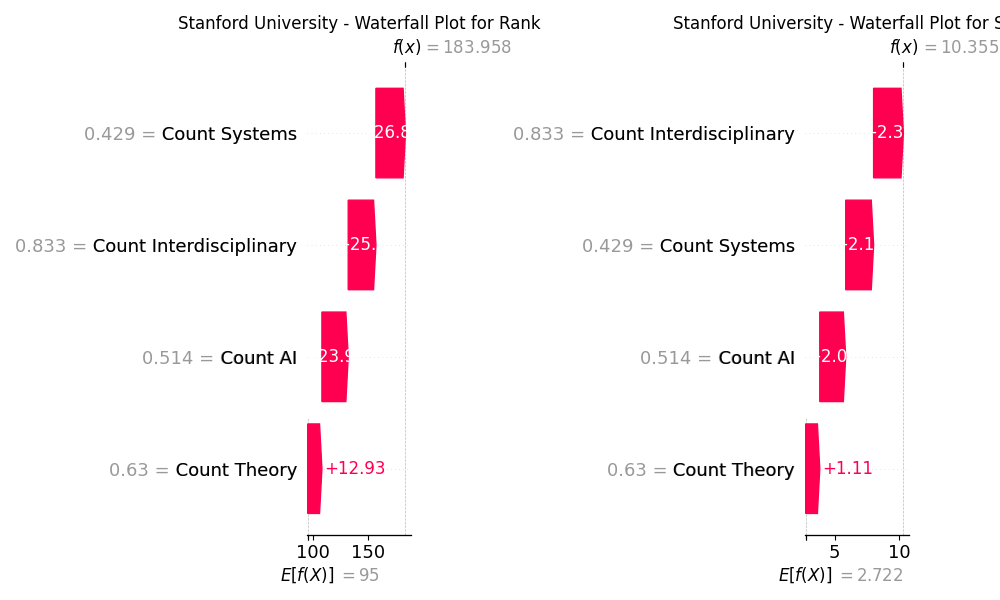
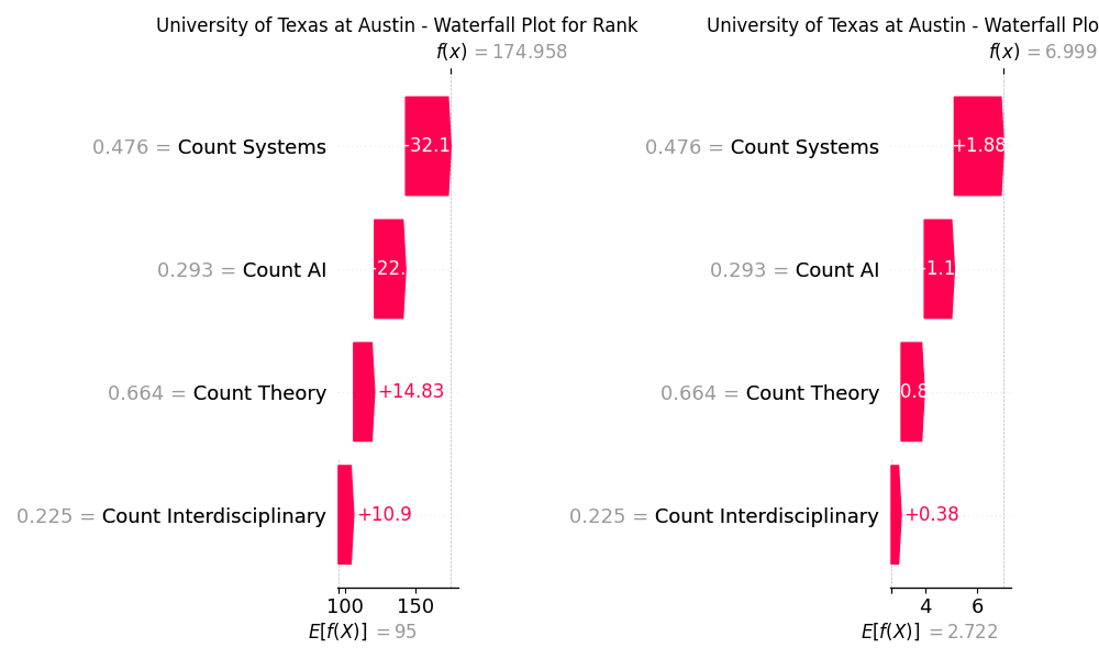
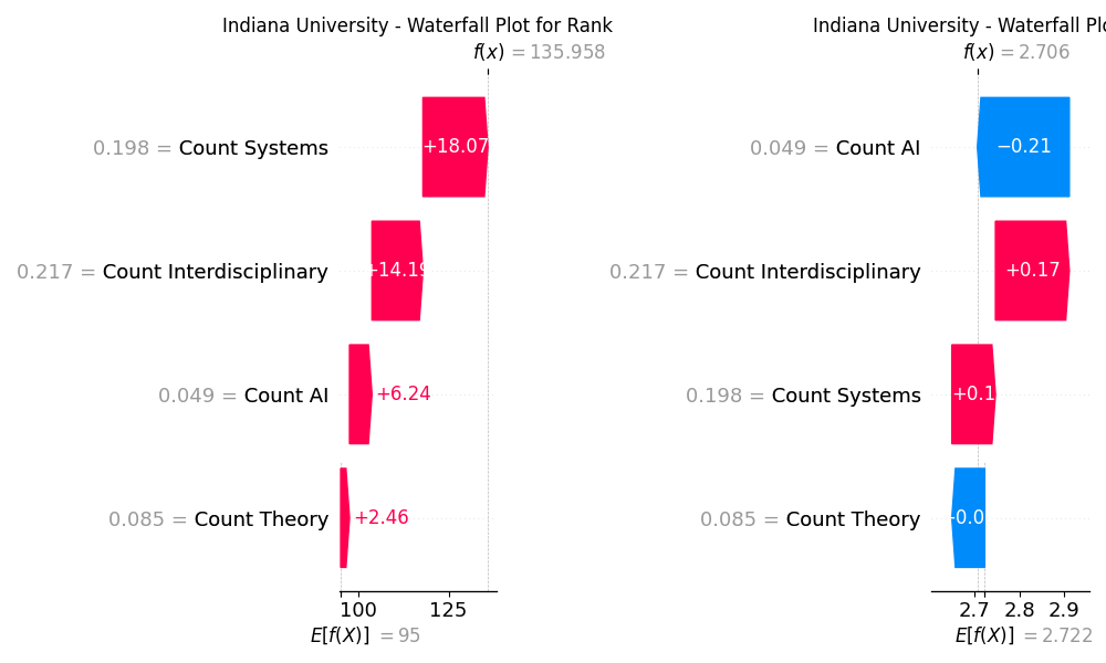
As the result we see that for each university, the importance of features for each QOI may be either very similar or differ a lot. For Stanford University, the feature Systems is the most impactful for rank and is followed by the feature Interdisciplinary, while for score, it’s vice versa. For University of Texas, the features have the same order of importance for both its QOIs, and all of them contribute to improving the score/rank of the university. On the contrary, for Indiana University, while the order of features by their importance is the same as for Stanford University for rank QOI, in the case of score, features AI and Theory contribute negatively, and AI is the most impactful feature.