Basic usage

This example shows a simple application of ShaRP over a toy dataset.

We will start by setting up the imports, environment variables and a basic score function that will be used to determine rankings.

import numpy as np
import matplotlib.pyplot as plt
from sklearn.utils import check_random_state
from sharp import ShaRP
from sharp.utils import scores_to_ordering

# Set up some envrionment variables
RNG_SEED = 42
N_SAMPLES = 50
rng = check_random_state(RNG_SEED)


def score_function(X):
    return 0.5 * X[:, 0] + 0.5 * X[:, 1]

We can now generate a simple mock dataset with 2 features, one sampled from a normal distribution, another from a bernoulli.

X = np.concatenate(
    [rng.normal(size=(N_SAMPLES, 1)), rng.binomial(1, 0.5, size=(N_SAMPLES, 1))], axis=1
)
y = score_function(X)
rank = scores_to_ordering(y)

Next, we will set up ShaRP:

xai = ShaRP(
    qoi="rank",
    target_function=score_function,
    measure="shapley",
    sample_size=None,
    replace=False,
    random_state=RNG_SEED,
)
xai.fit(X)

Let’s take a look at some shapley values used for ranking explanations:

print("Aggregate contribution of a single feature:", xai.feature(0, X))
print("Aggregate feature contributions:", xai.all(X).mean(axis=0))

individual_scores = xai.individual(9, X)
print("Feature contributions to a single observation: ", individual_scores)

pair_scores = xai.pairwise(X[2], X[3])
print("Pairwise comparison (one vs one):", pair_scores)

print("Pairwise comparison (one vs group):", xai.pairwise(X[2], X[5:10]))

Aggregate contribution of a single feature: 0.0
Aggregate feature contributions: [0. 0.]
Feature contributions to a single observation:  [np.float64(12.14), np.float64(6.359999999999999)]
Pairwise comparison (one vs one): [np.float64(-7.5), np.float64(-9.5)]
Pairwise comparison (one vs group): [np.float64(4.3), np.float64(-7.699999999999999)]

We can also turn these into visualizations:

plt.style.use("seaborn-v0_8-whitegrid")

# Visualization of feature contributions
print("Sample 2 feature values:", X[2])
print("Sample 3 feature values:", X[3])
fig, axes = plt.subplots(1, 2, figsize=(13.5, 4.5), layout="constrained")

# Bar plot comparing two points
xai.plot.bar(pair_scores, ax=axes[0], color="#ff0051")
axes[0].set_title(
    f"Pairwise comparison - Sample 2 (rank {rank[2]}) vs 3 (rank {rank[3]})",
    fontsize=12,
    y=-0.2,
)
axes[0].set_xlabel("")
axes[0].set_ylabel("Contribution to rank", fontsize=12)
axes[0].tick_params(axis="both", which="major", labelsize=12)

# Waterfall explaining rank for sample 2
axes[1] = xai.plot.waterfall(
    individual_scores, feature_values=X[9], mean_target_value=rank.mean()
)
ax = axes[1].gca()
ax.set_title("Rank explanation for Sample 9", fontsize=12, y=-0.2)

plt.show()

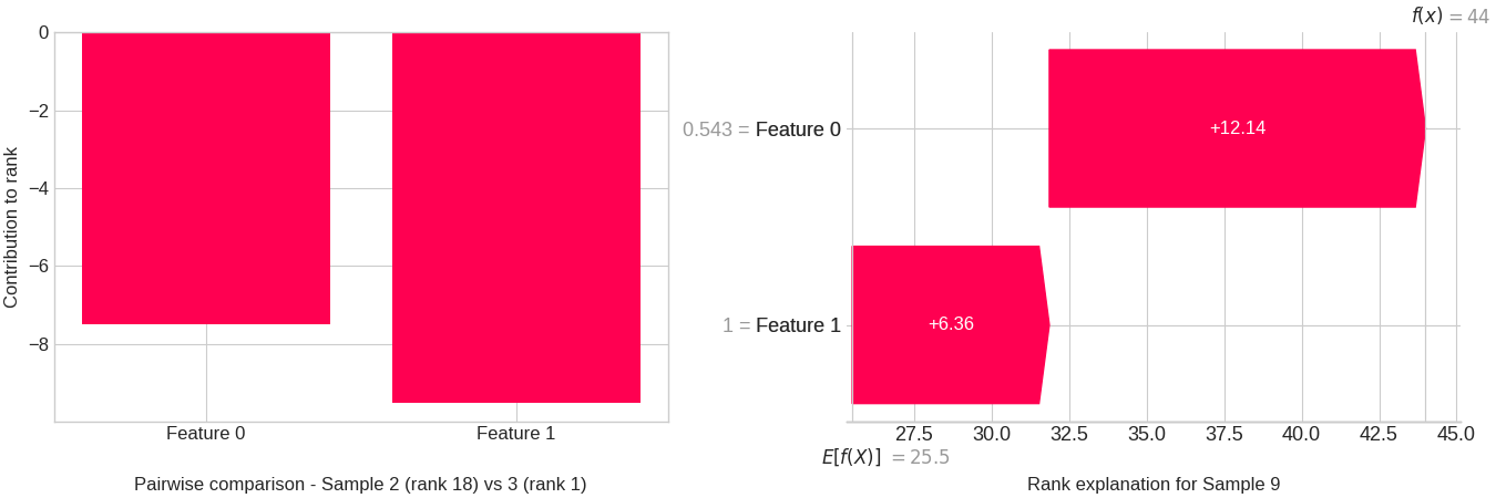
Sample 2 feature values: [0.64768854 0.        ]
Sample 3 feature values: [1.52302986 1.        ]