Note
Go to the end to download the full example code.
ShaRP for classification on large datasets with mixed data types
This example showcases a more complex setting, where we will develop and interpret a classification model using a larger dataset with both categorical and continuous features.
sharp is designed to operate over the unprocessed input space, to ensure every
“Frankenstein” point generated to compute feature contributions are plausible. This means
that the function producing the scores (or class predictions) should take as input the
raw dataset, and every preprocessing step leading to the black box predictions/scores
should be included within it.
We will start by downloading the German Credit dataset.
import pandas as pd
import matplotlib.pyplot as plt
from sklearn.datasets import fetch_openml
from sklearn.model_selection import train_test_split
from sklearn.preprocessing import OneHotEncoder, MinMaxScaler
from sklearn.compose import ColumnTransformer
from sklearn.linear_model import LogisticRegression
from sklearn.pipeline import make_pipeline
from sharp import ShaRP
Let’s get the data first. We will use the dataset that classifies people described by a set of attributes as good or bad credit risks.
df = fetch_openml(data_id=31, parser="auto")["frame"]
df.head(5)
Split X and y (input and target) from df and split train and test:
X = df.drop(columns="class")
y = df["class"]

categorical_features = X.dtypes.apply(
    lambda dtype: isinstance(dtype, pd.CategoricalDtype)
).values

X_train, X_test, y_train, y_test = train_test_split(
    X, y, test_size=0.1, random_state=42
)
Now we will set up model. Here, we will use a pipeline to combine all the preprocessing
steps. However, to use sharp, it is also sufficient to pass any function
(containing all the preprocessing steps) that takes a numpy array as input and outputs
the model’s predictions.
transformer = ColumnTransformer(
    transformers=[
        ("onehot", OneHotEncoder(sparse_output=False), categorical_features),
        ("minmax", MinMaxScaler(), ~categorical_features),
    ],
    remainder="passthrough",
    n_jobs=-1,
)
classifier = LogisticRegression(random_state=42)
model = make_pipeline(transformer, classifier)
model.fit(X_train.values, y_train.values)
We can now use sharp to explain our model’s predictions! If we consider the dataset
to be too large, we have a few options to reduce computational complexity, such as
configuring the n_jobs parameter, setting a value on sample_size, or setting
measure=unary.
xai = ShaRP(
    qoi="flip",
    target_function=model.predict,
    measure="unary",
    sample_size=None,
    random_state=42,
    n_jobs=-1,
    verbose=1,
)
xai.fit(X_test)

unary_values = pd.DataFrame(xai.all(X_test), columns=X.columns)
unary_values
  0%|          | 0/2000 [00:00<?, ?it/s]
  0%|          | 1/2000 [00:00<08:50,  3.77it/s]
  0%|          | 3/2000 [00:00<03:42,  8.99it/s]
  0%|          | 5/2000 [00:00<03:08, 10.57it/s]
  0%|          | 7/2000 [00:00<02:44, 12.14it/s]
  0%|          | 9/2000 [00:00<02:36, 12.75it/s]
  1%|          | 11/2000 [00:01<04:10,  7.92it/s]
  1%|          | 14/2000 [00:01<02:58, 11.10it/s]
  1%|          | 20/2000 [00:01<01:45, 18.73it/s]
  1%|          | 23/2000 [00:01<01:41, 19.43it/s]
  1%|▏         | 26/2000 [00:01<01:34, 20.97it/s]
  2%|▏         | 31/2000 [00:01<01:13, 26.94it/s]
  2%|▏         | 35/2000 [00:01<01:09, 28.22it/s]
  2%|▏         | 39/2000 [00:02<01:06, 29.49it/s]
  2%|▏         | 43/2000 [00:02<01:19, 24.69it/s]
  2%|▏         | 47/2000 [00:02<01:14, 26.12it/s]
  3%|▎         | 51/2000 [00:02<01:27, 22.28it/s]
  3%|▎         | 54/2000 [00:02<01:34, 20.62it/s]
  3%|▎         | 58/2000 [00:03<01:26, 22.58it/s]
  3%|▎         | 62/2000 [00:03<01:33, 20.78it/s]
  3%|▎         | 66/2000 [00:03<01:23, 23.22it/s]
  4%|▎         | 70/2000 [00:03<01:24, 22.91it/s]
  4%|▎         | 74/2000 [00:03<01:21, 23.65it/s]
  4%|▍         | 78/2000 [00:03<01:23, 22.95it/s]
  4%|▍         | 82/2000 [00:04<01:26, 22.13it/s]
  4%|▍         | 86/2000 [00:04<01:18, 24.54it/s]
  4%|▍         | 90/2000 [00:04<01:15, 25.37it/s]
  5%|▍         | 94/2000 [00:04<01:14, 25.44it/s]
  5%|▍         | 98/2000 [00:04<01:23, 22.72it/s]
  5%|▌         | 102/2000 [00:04<01:19, 23.83it/s]
  5%|▌         | 106/2000 [00:05<01:13, 25.89it/s]
  6%|▌         | 110/2000 [00:05<01:17, 24.36it/s]
  6%|▌         | 114/2000 [00:05<01:14, 25.39it/s]
  6%|▌         | 118/2000 [00:05<01:19, 23.65it/s]
  6%|▌         | 122/2000 [00:05<01:24, 22.30it/s]
  6%|▋         | 126/2000 [00:05<01:16, 24.65it/s]
  6%|▋         | 130/2000 [00:06<01:17, 24.08it/s]
  7%|▋         | 134/2000 [00:06<01:12, 25.87it/s]
  7%|▋         | 138/2000 [00:06<01:19, 23.28it/s]
  7%|▋         | 142/2000 [00:06<01:22, 22.62it/s]
  7%|▋         | 146/2000 [00:06<01:15, 24.65it/s]
  8%|▊         | 150/2000 [00:06<01:16, 24.25it/s]
  8%|▊         | 154/2000 [00:07<01:12, 25.37it/s]
  8%|▊         | 158/2000 [00:07<01:21, 22.57it/s]
  8%|▊         | 162/2000 [00:07<01:22, 22.37it/s]
  8%|▊         | 166/2000 [00:07<01:13, 25.01it/s]
  8%|▊         | 170/2000 [00:07<01:12, 25.36it/s]
  9%|▊         | 174/2000 [00:07<01:08, 26.78it/s]
  9%|▉         | 178/2000 [00:08<01:20, 22.53it/s]
  9%|▉         | 182/2000 [00:08<01:20, 22.61it/s]
  9%|▉         | 186/2000 [00:08<01:12, 24.96it/s]
 10%|▉         | 190/2000 [00:08<01:10, 25.55it/s]
 10%|▉         | 194/2000 [00:08<01:14, 24.25it/s]
 10%|▉         | 198/2000 [00:08<01:17, 23.34it/s]
 10%|█         | 202/2000 [00:09<01:18, 23.03it/s]
 10%|█         | 206/2000 [00:09<01:10, 25.43it/s]
 10%|█         | 210/2000 [00:09<01:10, 25.36it/s]
 11%|█         | 214/2000 [00:09<01:12, 24.60it/s]
 11%|█         | 218/2000 [00:09<01:21, 21.98it/s]
 11%|█         | 222/2000 [00:09<01:16, 23.29it/s]
 11%|█▏        | 226/2000 [00:10<01:09, 25.58it/s]
 12%|█▏        | 230/2000 [00:10<01:06, 26.49it/s]
 12%|█▏        | 234/2000 [00:10<01:11, 24.79it/s]
 12%|█▏        | 238/2000 [00:10<01:16, 23.06it/s]
 12%|█▏        | 242/2000 [00:10<01:17, 22.57it/s]
 12%|█▏        | 246/2000 [00:10<01:11, 24.68it/s]
 12%|█▎        | 250/2000 [00:11<01:13, 23.74it/s]
 13%|█▎        | 254/2000 [00:11<01:11, 24.57it/s]
 13%|█▎        | 258/2000 [00:11<01:15, 23.00it/s]
 13%|█▎        | 262/2000 [00:11<01:19, 21.97it/s]
 13%|█▎        | 266/2000 [00:11<01:11, 24.35it/s]
 14%|█▎        | 270/2000 [00:11<01:08, 25.15it/s]
 14%|█▎        | 274/2000 [00:12<01:09, 24.83it/s]
 14%|█▍        | 278/2000 [00:12<01:15, 22.82it/s]
 14%|█▍        | 282/2000 [00:12<01:16, 22.33it/s]
 14%|█▍        | 286/2000 [00:12<01:08, 24.87it/s]
 14%|█▍        | 290/2000 [00:12<01:06, 25.89it/s]
 15%|█▍        | 294/2000 [00:12<01:04, 26.50it/s]
 15%|█▍        | 298/2000 [00:13<01:15, 22.53it/s]
 15%|█▌        | 302/2000 [00:13<01:13, 23.25it/s]
 15%|█▌        | 306/2000 [00:13<01:05, 25.78it/s]
 16%|█▌        | 310/2000 [00:13<01:06, 25.56it/s]
 16%|█▌        | 314/2000 [00:13<01:04, 26.11it/s]
 16%|█▌        | 318/2000 [00:13<01:11, 23.51it/s]
 16%|█▌        | 322/2000 [00:14<01:12, 23.22it/s]
 16%|█▋        | 326/2000 [00:14<01:05, 25.67it/s]
 16%|█▋        | 330/2000 [00:14<01:06, 25.18it/s]
 17%|█▋        | 334/2000 [00:14<01:06, 24.90it/s]
 17%|█▋        | 338/2000 [00:14<01:14, 22.43it/s]
 17%|█▋        | 342/2000 [00:14<01:12, 22.94it/s]
 17%|█▋        | 346/2000 [00:14<01:05, 25.34it/s]
 18%|█▊        | 350/2000 [00:15<01:04, 25.46it/s]
 18%|█▊        | 354/2000 [00:15<01:02, 26.25it/s]
 18%|█▊        | 358/2000 [00:15<01:11, 23.10it/s]
 18%|█▊        | 362/2000 [00:15<01:11, 22.89it/s]
 18%|█▊        | 366/2000 [00:15<01:05, 24.93it/s]
 18%|█▊        | 370/2000 [00:15<01:05, 24.73it/s]
 19%|█▊        | 374/2000 [00:16<01:06, 24.40it/s]
 19%|█▉        | 378/2000 [00:16<01:10, 22.88it/s]
 19%|█▉        | 382/2000 [00:16<01:11, 22.51it/s]
 19%|█▉        | 386/2000 [00:16<01:04, 24.88it/s]
 20%|█▉        | 390/2000 [00:16<01:05, 24.41it/s]
 20%|█▉        | 394/2000 [00:16<01:05, 24.46it/s]
 20%|█▉        | 398/2000 [00:17<01:11, 22.49it/s]
 20%|██        | 402/2000 [00:17<01:09, 22.91it/s]
 20%|██        | 406/2000 [00:17<01:03, 25.18it/s]
 20%|██        | 410/2000 [00:17<01:01, 26.05it/s]
 21%|██        | 414/2000 [00:17<01:05, 24.36it/s]
 21%|██        | 418/2000 [00:18<01:09, 22.75it/s]
 21%|██        | 422/2000 [00:18<01:10, 22.32it/s]
 21%|██▏       | 426/2000 [00:18<01:03, 24.68it/s]
 22%|██▏       | 430/2000 [00:18<01:02, 25.28it/s]
 22%|██▏       | 434/2000 [00:18<01:02, 25.14it/s]
 22%|██▏       | 438/2000 [00:18<01:08, 22.90it/s]
 22%|██▏       | 442/2000 [00:19<01:09, 22.55it/s]
 22%|██▏       | 446/2000 [00:19<01:03, 24.55it/s]
 22%|██▎       | 450/2000 [00:19<01:03, 24.46it/s]
 23%|██▎       | 454/2000 [00:19<01:00, 25.39it/s]
 23%|██▎       | 458/2000 [00:19<01:07, 22.79it/s]
 23%|██▎       | 462/2000 [00:19<01:09, 22.27it/s]
 23%|██▎       | 466/2000 [00:19<01:01, 25.09it/s]
 24%|██▎       | 470/2000 [00:20<00:59, 25.62it/s]
 24%|██▎       | 474/2000 [00:20<01:01, 25.00it/s]
 24%|██▍       | 478/2000 [00:20<01:07, 22.68it/s]
 24%|██▍       | 482/2000 [00:20<01:09, 21.98it/s]
 24%|██▍       | 486/2000 [00:20<01:02, 24.13it/s]
 24%|██▍       | 490/2000 [00:20<01:00, 25.10it/s]
 25%|██▍       | 494/2000 [00:21<00:58, 25.94it/s]
 25%|██▍       | 498/2000 [00:21<01:07, 22.15it/s]
 25%|██▌       | 502/2000 [00:21<01:06, 22.48it/s]
 25%|██▌       | 506/2000 [00:21<01:00, 24.54it/s]
 26%|██▌       | 510/2000 [00:21<01:01, 24.20it/s]
 26%|██▌       | 514/2000 [00:21<01:01, 24.19it/s]
 26%|██▌       | 518/2000 [00:22<01:03, 23.48it/s]
 26%|██▌       | 522/2000 [00:22<01:06, 22.36it/s]
 26%|██▋       | 526/2000 [00:22<00:59, 24.87it/s]
 26%|██▋       | 530/2000 [00:22<00:57, 25.48it/s]
 27%|██▋       | 534/2000 [00:22<00:57, 25.34it/s]
 27%|██▋       | 538/2000 [00:23<01:04, 22.62it/s]
 27%|██▋       | 542/2000 [00:23<01:04, 22.71it/s]
 27%|██▋       | 546/2000 [00:23<00:58, 24.80it/s]
 28%|██▊       | 550/2000 [00:23<00:57, 25.36it/s]
 28%|██▊       | 554/2000 [00:23<00:58, 24.87it/s]
 28%|██▊       | 558/2000 [00:23<01:02, 23.04it/s]
 28%|██▊       | 562/2000 [00:24<01:02, 22.98it/s]
 28%|██▊       | 566/2000 [00:24<00:57, 24.87it/s]
 28%|██▊       | 570/2000 [00:24<00:57, 24.70it/s]
 29%|██▊       | 574/2000 [00:24<00:56, 25.46it/s]
 29%|██▉       | 578/2000 [00:24<01:02, 22.66it/s]
 29%|██▉       | 582/2000 [00:24<01:01, 22.92it/s]
 29%|██▉       | 586/2000 [00:24<00:55, 25.27it/s]
 30%|██▉       | 590/2000 [00:25<00:53, 26.13it/s]
 30%|██▉       | 594/2000 [00:25<00:57, 24.54it/s]
 30%|██▉       | 598/2000 [00:25<01:00, 23.12it/s]
 30%|███       | 602/2000 [00:25<00:58, 23.78it/s]
 30%|███       | 606/2000 [00:25<00:56, 24.51it/s]
 30%|███       | 610/2000 [00:25<00:54, 25.58it/s]
 31%|███       | 614/2000 [00:26<00:55, 25.02it/s]
 31%|███       | 618/2000 [00:26<01:01, 22.64it/s]
 31%|███       | 622/2000 [00:26<00:59, 23.27it/s]
 31%|███▏      | 626/2000 [00:26<00:54, 25.21it/s]
 32%|███▏      | 630/2000 [00:26<00:52, 26.02it/s]
 32%|███▏      | 634/2000 [00:26<00:55, 24.43it/s]
 32%|███▏      | 638/2000 [00:27<00:58, 23.18it/s]
 32%|███▏      | 642/2000 [00:27<00:57, 23.43it/s]
 32%|███▏      | 646/2000 [00:27<00:57, 23.37it/s]
 32%|███▎      | 650/2000 [00:27<00:54, 24.77it/s]
 33%|███▎      | 654/2000 [00:27<00:52, 25.49it/s]
 33%|███▎      | 658/2000 [00:28<01:01, 21.92it/s]
 33%|███▎      | 662/2000 [00:28<00:58, 22.87it/s]
 33%|███▎      | 666/2000 [00:28<00:52, 25.22it/s]
 34%|███▎      | 670/2000 [00:28<00:51, 25.86it/s]
 34%|███▎      | 674/2000 [00:28<00:54, 24.40it/s]
 34%|███▍      | 678/2000 [00:28<00:56, 23.30it/s]
 34%|███▍      | 682/2000 [00:29<00:59, 22.05it/s]
 34%|███▍      | 686/2000 [00:29<00:53, 24.36it/s]
 34%|███▍      | 690/2000 [00:29<00:52, 25.09it/s]
 35%|███▍      | 694/2000 [00:29<00:50, 25.81it/s]
 35%|███▍      | 698/2000 [00:29<00:58, 22.27it/s]
 35%|███▌      | 702/2000 [00:29<00:57, 22.72it/s]
 35%|███▌      | 706/2000 [00:29<00:54, 23.93it/s]
 36%|███▌      | 710/2000 [00:30<00:52, 24.49it/s]
 36%|███▌      | 714/2000 [00:30<00:47, 27.14it/s]
 36%|███▌      | 718/2000 [00:30<00:58, 21.81it/s]
 36%|███▌      | 722/2000 [00:30<00:54, 23.62it/s]
 36%|███▋      | 726/2000 [00:30<00:49, 25.83it/s]
 36%|███▋      | 730/2000 [00:30<00:47, 26.46it/s]
 37%|███▋      | 734/2000 [00:31<00:52, 23.92it/s]
 37%|███▋      | 738/2000 [00:31<00:52, 23.91it/s]
 37%|███▋      | 742/2000 [00:31<00:56, 22.17it/s]
 37%|███▋      | 746/2000 [00:31<00:50, 24.84it/s]
 38%|███▊      | 750/2000 [00:31<00:48, 25.82it/s]
 38%|███▊      | 754/2000 [00:31<00:51, 24.35it/s]
 38%|███▊      | 758/2000 [00:32<00:54, 22.62it/s]
 38%|███▊      | 762/2000 [00:32<00:53, 23.18it/s]
 38%|███▊      | 766/2000 [00:32<00:51, 23.93it/s]
 38%|███▊      | 770/2000 [00:32<00:49, 24.80it/s]
 39%|███▊      | 774/2000 [00:32<00:45, 27.05it/s]
 39%|███▉      | 778/2000 [00:32<00:55, 22.16it/s]
 39%|███▉      | 782/2000 [00:33<00:51, 23.59it/s]
 39%|███▉      | 786/2000 [00:33<00:47, 25.77it/s]
 40%|███▉      | 790/2000 [00:33<00:45, 26.60it/s]
 40%|███▉      | 794/2000 [00:33<00:48, 24.63it/s]
 40%|███▉      | 798/2000 [00:33<00:52, 22.95it/s]
 40%|████      | 802/2000 [00:33<00:54, 22.02it/s]
 40%|████      | 806/2000 [00:34<00:48, 24.42it/s]
 40%|████      | 810/2000 [00:34<00:46, 25.40it/s]
 41%|████      | 814/2000 [00:34<00:48, 24.58it/s]
 41%|████      | 818/2000 [00:34<00:51, 22.98it/s]
 41%|████      | 822/2000 [00:34<00:51, 23.02it/s]
 41%|████▏     | 826/2000 [00:34<00:46, 25.07it/s]
 42%|████▏     | 830/2000 [00:35<00:47, 24.40it/s]
 42%|████▏     | 834/2000 [00:35<00:48, 24.06it/s]
 42%|████▏     | 838/2000 [00:35<00:48, 23.85it/s]
 42%|████▏     | 842/2000 [00:35<00:52, 22.22it/s]
 42%|████▏     | 846/2000 [00:35<00:46, 24.72it/s]
 42%|████▎     | 850/2000 [00:35<00:44, 25.60it/s]
 43%|████▎     | 854/2000 [00:36<00:44, 25.79it/s]
 43%|████▎     | 858/2000 [00:36<00:50, 22.65it/s]
 43%|████▎     | 862/2000 [00:36<00:49, 22.93it/s]
 43%|████▎     | 866/2000 [00:36<00:46, 24.29it/s]
 44%|████▎     | 870/2000 [00:36<00:46, 24.36it/s]
 44%|████▎     | 874/2000 [00:36<00:43, 25.83it/s]
 44%|████▍     | 878/2000 [00:37<00:49, 22.68it/s]
 44%|████▍     | 882/2000 [00:37<00:48, 22.83it/s]
 44%|████▍     | 886/2000 [00:37<00:44, 25.13it/s]
 44%|████▍     | 890/2000 [00:37<00:43, 25.76it/s]
 45%|████▍     | 894/2000 [00:37<00:45, 24.39it/s]
 45%|████▍     | 898/2000 [00:37<00:47, 23.21it/s]
 45%|████▌     | 902/2000 [00:38<00:46, 23.48it/s]
 45%|████▌     | 906/2000 [00:38<00:45, 24.18it/s]
 46%|████▌     | 910/2000 [00:38<00:43, 25.04it/s]
 46%|████▌     | 914/2000 [00:38<00:42, 25.74it/s]
 46%|████▌     | 918/2000 [00:38<00:48, 22.30it/s]
 46%|████▌     | 922/2000 [00:38<00:46, 22.97it/s]
 46%|████▋     | 926/2000 [00:39<00:42, 25.21it/s]
 46%|████▋     | 930/2000 [00:39<00:40, 26.29it/s]
 47%|████▋     | 934/2000 [00:39<00:45, 23.36it/s]
 47%|████▋     | 938/2000 [00:39<00:46, 22.87it/s]
 47%|████▋     | 942/2000 [00:39<00:48, 21.95it/s]
 47%|████▋     | 946/2000 [00:39<00:43, 24.13it/s]
 48%|████▊     | 950/2000 [00:40<00:41, 25.55it/s]
 48%|████▊     | 954/2000 [00:40<00:40, 26.14it/s]
 48%|████▊     | 958/2000 [00:40<00:47, 22.07it/s]
 48%|████▊     | 962/2000 [00:40<00:44, 23.31it/s]
 48%|████▊     | 966/2000 [00:40<00:44, 22.98it/s]
 48%|████▊     | 970/2000 [00:40<00:42, 24.39it/s]
 49%|████▊     | 974/2000 [00:41<00:40, 25.17it/s]
 49%|████▉     | 978/2000 [00:41<00:46, 21.89it/s]
 49%|████▉     | 982/2000 [00:41<00:43, 23.22it/s]
 49%|████▉     | 986/2000 [00:41<00:39, 25.60it/s]
 50%|████▉     | 990/2000 [00:41<00:38, 26.05it/s]
 50%|████▉     | 994/2000 [00:41<00:38, 26.45it/s]
 50%|████▉     | 998/2000 [00:42<00:43, 22.96it/s]
 50%|█████     | 1002/2000 [00:42<00:43, 23.04it/s]
 50%|█████     | 1006/2000 [00:42<00:40, 24.47it/s]
 50%|█████     | 1010/2000 [00:42<00:40, 24.59it/s]
 51%|█████     | 1014/2000 [00:42<00:40, 24.49it/s]
 51%|█████     | 1018/2000 [00:42<00:42, 23.02it/s]
 51%|█████     | 1022/2000 [00:43<00:43, 22.71it/s]
 51%|█████▏    | 1026/2000 [00:43<00:38, 25.13it/s]
 52%|█████▏    | 1030/2000 [00:43<00:37, 26.05it/s]
 52%|█████▏    | 1034/2000 [00:43<00:38, 24.86it/s]
 52%|█████▏    | 1038/2000 [00:43<00:42, 22.60it/s]
 52%|█████▏    | 1042/2000 [00:43<00:43, 22.15it/s]
 52%|█████▏    | 1046/2000 [00:44<00:39, 24.06it/s]
 52%|█████▎    | 1050/2000 [00:44<00:37, 25.55it/s]
 53%|█████▎    | 1054/2000 [00:44<00:36, 25.91it/s]
 53%|█████▎    | 1058/2000 [00:44<00:42, 22.01it/s]
 53%|█████▎    | 1062/2000 [00:44<00:40, 22.98it/s]
 53%|█████▎    | 1066/2000 [00:44<00:38, 23.98it/s]
 54%|█████▎    | 1070/2000 [00:45<00:37, 24.61it/s]
 54%|█████▎    | 1074/2000 [00:45<00:35, 26.32it/s]
 54%|█████▍    | 1078/2000 [00:45<00:41, 22.31it/s]
 54%|█████▍    | 1082/2000 [00:45<00:39, 23.22it/s]
 54%|█████▍    | 1086/2000 [00:45<00:35, 25.70it/s]
 55%|█████▍    | 1090/2000 [00:45<00:34, 26.38it/s]
 55%|█████▍    | 1094/2000 [00:46<00:36, 24.63it/s]
 55%|█████▍    | 1098/2000 [00:46<00:39, 23.09it/s]
 55%|█████▌    | 1102/2000 [00:46<00:38, 23.45it/s]
 55%|█████▌    | 1106/2000 [00:46<00:36, 24.33it/s]
 56%|█████▌    | 1110/2000 [00:46<00:35, 25.33it/s]
 56%|█████▌    | 1114/2000 [00:46<00:35, 24.74it/s]
 56%|█████▌    | 1118/2000 [00:47<00:37, 23.27it/s]
 56%|█████▌    | 1122/2000 [00:47<00:37, 23.39it/s]
 56%|█████▋    | 1126/2000 [00:47<00:34, 25.52it/s]
 56%|█████▋    | 1130/2000 [00:47<00:33, 25.98it/s]
 57%|█████▋    | 1134/2000 [00:47<00:36, 23.74it/s]
 57%|█████▋    | 1138/2000 [00:47<00:37, 23.27it/s]
 57%|█████▋    | 1142/2000 [00:48<00:39, 21.88it/s]
 57%|█████▋    | 1146/2000 [00:48<00:35, 24.30it/s]
 57%|█████▊    | 1150/2000 [00:48<00:33, 25.71it/s]
 58%|█████▊    | 1154/2000 [00:48<00:32, 26.06it/s]
 58%|█████▊    | 1158/2000 [00:48<00:38, 22.16it/s]
 58%|█████▊    | 1162/2000 [00:48<00:36, 23.04it/s]
 58%|█████▊    | 1166/2000 [00:49<00:33, 24.87it/s]
 58%|█████▊    | 1170/2000 [00:49<00:34, 23.99it/s]
 59%|█████▊    | 1174/2000 [00:49<00:30, 26.89it/s]
 59%|█████▉    | 1178/2000 [00:49<00:36, 22.75it/s]
 59%|█████▉    | 1182/2000 [00:49<00:34, 23.54it/s]
 59%|█████▉    | 1186/2000 [00:49<00:31, 25.73it/s]
 60%|█████▉    | 1190/2000 [00:50<00:31, 25.38it/s]
 60%|█████▉    | 1194/2000 [00:50<00:33, 24.32it/s]
 60%|█████▉    | 1198/2000 [00:50<00:33, 23.64it/s]
 60%|██████    | 1202/2000 [00:50<00:34, 23.07it/s]
 60%|██████    | 1206/2000 [00:50<00:31, 25.19it/s]
 60%|██████    | 1210/2000 [00:50<00:32, 23.97it/s]
 61%|██████    | 1214/2000 [00:51<00:32, 23.88it/s]
 61%|██████    | 1218/2000 [00:51<00:34, 22.71it/s]
 61%|██████    | 1222/2000 [00:51<00:34, 22.56it/s]
 61%|██████▏   | 1226/2000 [00:51<00:31, 24.69it/s]
 62%|██████▏   | 1230/2000 [00:51<00:32, 23.48it/s]
 62%|██████▏   | 1234/2000 [00:51<00:28, 26.50it/s]
 62%|██████▏   | 1238/2000 [00:52<00:32, 23.21it/s]
 62%|██████▏   | 1242/2000 [00:52<00:32, 23.48it/s]
 62%|██████▏   | 1246/2000 [00:52<00:29, 25.88it/s]
 62%|██████▎   | 1250/2000 [00:52<00:29, 25.82it/s]
 63%|██████▎   | 1254/2000 [00:52<00:29, 25.31it/s]
 63%|██████▎   | 1258/2000 [00:52<00:32, 23.17it/s]
 63%|██████▎   | 1262/2000 [00:53<00:32, 22.47it/s]
 63%|██████▎   | 1266/2000 [00:53<00:29, 24.92it/s]
 64%|██████▎   | 1270/2000 [00:53<00:28, 25.59it/s]
 64%|██████▎   | 1274/2000 [00:53<00:28, 25.67it/s]
 64%|██████▍   | 1278/2000 [00:53<00:31, 22.78it/s]
 64%|██████▍   | 1282/2000 [00:53<00:31, 22.92it/s]
 64%|██████▍   | 1286/2000 [00:54<00:29, 24.41it/s]
 64%|██████▍   | 1290/2000 [00:54<00:29, 24.38it/s]
 65%|██████▍   | 1294/2000 [00:54<00:29, 23.88it/s]
 65%|██████▍   | 1298/2000 [00:54<00:30, 22.73it/s]
 65%|██████▌   | 1302/2000 [00:54<00:30, 22.64it/s]
 65%|██████▌   | 1306/2000 [00:54<00:28, 24.67it/s]
 66%|██████▌   | 1310/2000 [00:54<00:26, 25.89it/s]
 66%|██████▌   | 1314/2000 [00:55<00:27, 24.59it/s]
 66%|██████▌   | 1318/2000 [00:55<00:30, 22.52it/s]
 66%|██████▌   | 1322/2000 [00:55<00:29, 23.13it/s]
 66%|██████▋   | 1326/2000 [00:55<00:28, 23.80it/s]
 66%|██████▋   | 1330/2000 [00:55<00:26, 24.90it/s]
 67%|██████▋   | 1334/2000 [00:55<00:25, 26.00it/s]
 67%|██████▋   | 1338/2000 [00:56<00:29, 22.23it/s]
 67%|██████▋   | 1342/2000 [00:56<00:28, 23.35it/s]
 67%|██████▋   | 1346/2000 [00:56<00:25, 25.62it/s]
 68%|██████▊   | 1350/2000 [00:56<00:24, 26.08it/s]
 68%|██████▊   | 1354/2000 [00:56<00:26, 24.70it/s]
 68%|██████▊   | 1358/2000 [00:57<00:27, 23.70it/s]
 68%|██████▊   | 1362/2000 [00:57<00:27, 22.98it/s]
 68%|██████▊   | 1366/2000 [00:57<00:25, 24.59it/s]
 68%|██████▊   | 1370/2000 [00:57<00:25, 24.55it/s]
 69%|██████▊   | 1374/2000 [00:57<00:25, 25.02it/s]
 69%|██████▉   | 1378/2000 [00:57<00:27, 22.64it/s]
 69%|██████▉   | 1382/2000 [00:58<00:27, 22.60it/s]
 69%|██████▉   | 1386/2000 [00:58<00:24, 24.90it/s]
 70%|██████▉   | 1390/2000 [00:58<00:23, 25.92it/s]
 70%|██████▉   | 1394/2000 [00:58<00:24, 24.46it/s]
 70%|██████▉   | 1398/2000 [00:58<00:26, 22.63it/s]
 70%|███████   | 1402/2000 [00:58<00:27, 22.05it/s]
 70%|███████   | 1406/2000 [00:59<00:24, 24.38it/s]
 70%|███████   | 1410/2000 [00:59<00:23, 25.55it/s]
 71%|███████   | 1414/2000 [00:59<00:23, 25.39it/s]
 71%|███████   | 1418/2000 [00:59<00:26, 22.29it/s]
 71%|███████   | 1422/2000 [00:59<00:25, 22.82it/s]
 71%|███████▏  | 1426/2000 [00:59<00:22, 25.08it/s]
 72%|███████▏  | 1430/2000 [00:59<00:22, 24.90it/s]
 72%|███████▏  | 1434/2000 [01:00<00:23, 23.98it/s]
 72%|███████▏  | 1438/2000 [01:00<00:25, 21.86it/s]
 72%|███████▏  | 1442/2000 [01:00<00:23, 23.27it/s]
 72%|███████▏  | 1446/2000 [01:00<00:21, 25.63it/s]
 72%|███████▎  | 1450/2000 [01:00<00:21, 25.58it/s]
 73%|███████▎  | 1454/2000 [01:00<00:21, 25.21it/s]
 73%|███████▎  | 1458/2000 [01:01<00:23, 23.44it/s]
 73%|███████▎  | 1462/2000 [01:01<00:23, 22.91it/s]
 73%|███████▎  | 1466/2000 [01:01<00:21, 24.96it/s]
 74%|███████▎  | 1470/2000 [01:01<00:21, 24.14it/s]
 74%|███████▎  | 1474/2000 [01:01<00:21, 24.44it/s]
 74%|███████▍  | 1478/2000 [01:02<00:22, 23.22it/s]
 74%|███████▍  | 1482/2000 [01:02<00:23, 22.36it/s]
 74%|███████▍  | 1486/2000 [01:02<00:20, 24.77it/s]
 74%|███████▍  | 1490/2000 [01:02<00:20, 24.92it/s]
 75%|███████▍  | 1494/2000 [01:02<00:20, 24.69it/s]
 75%|███████▍  | 1498/2000 [01:02<00:21, 23.06it/s]
 75%|███████▌  | 1502/2000 [01:03<00:22, 22.00it/s]
 75%|███████▌  | 1506/2000 [01:03<00:20, 24.31it/s]
 76%|███████▌  | 1510/2000 [01:03<00:19, 25.70it/s]
 76%|███████▌  | 1514/2000 [01:03<00:18, 26.83it/s]
 76%|███████▌  | 1518/2000 [01:03<00:21, 22.47it/s]
 76%|███████▌  | 1522/2000 [01:03<00:20, 23.32it/s]
 76%|███████▋  | 1526/2000 [01:03<00:18, 25.28it/s]
 76%|███████▋  | 1530/2000 [01:04<00:19, 24.05it/s]
 77%|███████▋  | 1534/2000 [01:04<00:17, 26.31it/s]
 77%|███████▋  | 1538/2000 [01:04<00:20, 22.79it/s]
 77%|███████▋  | 1542/2000 [01:04<00:19, 23.01it/s]
 77%|███████▋  | 1546/2000 [01:04<00:18, 25.21it/s]
 78%|███████▊  | 1550/2000 [01:04<00:17, 25.61it/s]
 78%|███████▊  | 1554/2000 [01:05<00:18, 24.14it/s]
 78%|███████▊  | 1558/2000 [01:05<00:18, 23.42it/s]
 78%|███████▊  | 1562/2000 [01:05<00:19, 22.78it/s]
 78%|███████▊  | 1566/2000 [01:05<00:17, 24.99it/s]
 78%|███████▊  | 1570/2000 [01:05<00:17, 24.12it/s]
 79%|███████▊  | 1574/2000 [01:05<00:17, 24.19it/s]
 79%|███████▉  | 1578/2000 [01:06<00:19, 21.53it/s]
 79%|███████▉  | 1582/2000 [01:06<00:18, 22.92it/s]
 79%|███████▉  | 1586/2000 [01:06<00:16, 24.61it/s]
 80%|███████▉  | 1590/2000 [01:06<00:16, 24.24it/s]
 80%|███████▉  | 1594/2000 [01:06<00:15, 26.76it/s]
 80%|███████▉  | 1598/2000 [01:07<00:17, 22.83it/s]
 80%|████████  | 1602/2000 [01:07<00:17, 23.19it/s]
 80%|████████  | 1606/2000 [01:07<00:15, 25.29it/s]
 80%|████████  | 1610/2000 [01:07<00:14, 26.11it/s]
 81%|████████  | 1614/2000 [01:07<00:16, 23.43it/s]
 81%|████████  | 1618/2000 [01:07<00:16, 23.30it/s]
 81%|████████  | 1622/2000 [01:08<00:17, 21.81it/s]
 81%|████████▏ | 1626/2000 [01:08<00:15, 24.57it/s]
 82%|████████▏ | 1630/2000 [01:08<00:14, 25.67it/s]
 82%|████████▏ | 1634/2000 [01:08<00:14, 25.46it/s]
 82%|████████▏ | 1638/2000 [01:08<00:16, 22.40it/s]
 82%|████████▏ | 1642/2000 [01:08<00:15, 23.02it/s]
 82%|████████▏ | 1646/2000 [01:08<00:14, 25.21it/s]
 82%|████████▎ | 1650/2000 [01:09<00:14, 24.62it/s]
 83%|████████▎ | 1654/2000 [01:09<00:14, 24.65it/s]
 83%|████████▎ | 1658/2000 [01:09<00:14, 23.66it/s]
 83%|████████▎ | 1662/2000 [01:09<00:14, 22.61it/s]
 83%|████████▎ | 1666/2000 [01:09<00:13, 25.29it/s]
 84%|████████▎ | 1670/2000 [01:09<00:12, 26.02it/s]
 84%|████████▎ | 1674/2000 [01:10<00:12, 25.40it/s]
 84%|████████▍ | 1678/2000 [01:10<00:14, 22.53it/s]
 84%|████████▍ | 1682/2000 [01:10<00:14, 22.40it/s]
 84%|████████▍ | 1686/2000 [01:10<00:12, 24.87it/s]
 84%|████████▍ | 1690/2000 [01:10<00:11, 25.84it/s]
 85%|████████▍ | 1694/2000 [01:10<00:11, 26.37it/s]
 85%|████████▍ | 1698/2000 [01:11<00:13, 22.69it/s]
 85%|████████▌ | 1702/2000 [01:11<00:12, 23.07it/s]
 85%|████████▌ | 1706/2000 [01:11<00:11, 24.52it/s]
 86%|████████▌ | 1710/2000 [01:11<00:11, 24.89it/s]
 86%|████████▌ | 1714/2000 [01:11<00:11, 25.47it/s]
 86%|████████▌ | 1718/2000 [01:11<00:12, 22.96it/s]
 86%|████████▌ | 1722/2000 [01:12<00:12, 22.57it/s]
 86%|████████▋ | 1726/2000 [01:12<00:11, 24.89it/s]
 86%|████████▋ | 1730/2000 [01:12<00:10, 25.77it/s]
 87%|████████▋ | 1734/2000 [01:12<00:11, 24.16it/s]
 87%|████████▋ | 1738/2000 [01:12<00:11, 23.21it/s]
 87%|████████▋ | 1742/2000 [01:13<00:11, 21.82it/s]
 87%|████████▋ | 1746/2000 [01:13<00:10, 24.29it/s]
 88%|████████▊ | 1750/2000 [01:13<00:09, 25.26it/s]
 88%|████████▊ | 1754/2000 [01:13<00:09, 26.64it/s]
 88%|████████▊ | 1758/2000 [01:13<00:11, 21.90it/s]
 88%|████████▊ | 1762/2000 [01:13<00:10, 22.99it/s]
 88%|████████▊ | 1766/2000 [01:13<00:09, 25.15it/s]
 88%|████████▊ | 1770/2000 [01:14<00:09, 24.55it/s]
 89%|████████▊ | 1774/2000 [01:14<00:08, 26.56it/s]
 89%|████████▉ | 1778/2000 [01:14<00:09, 22.59it/s]
 89%|████████▉ | 1782/2000 [01:14<00:09, 22.63it/s]
 89%|████████▉ | 1786/2000 [01:14<00:08, 24.92it/s]
 90%|████████▉ | 1790/2000 [01:14<00:08, 25.42it/s]
 90%|████████▉ | 1794/2000 [01:15<00:08, 24.15it/s]
 90%|████████▉ | 1798/2000 [01:15<00:08, 23.29it/s]
 90%|█████████ | 1802/2000 [01:15<00:08, 22.88it/s]
 90%|█████████ | 1806/2000 [01:15<00:07, 25.18it/s]
 90%|█████████ | 1810/2000 [01:15<00:07, 24.24it/s]
 91%|█████████ | 1814/2000 [01:15<00:07, 24.81it/s]
 91%|█████████ | 1818/2000 [01:16<00:08, 22.31it/s]
 91%|█████████ | 1822/2000 [01:16<00:07, 22.83it/s]
 91%|█████████▏| 1826/2000 [01:16<00:06, 24.96it/s]
 92%|█████████▏| 1830/2000 [01:16<00:07, 24.22it/s]
 92%|█████████▏| 1834/2000 [01:16<00:06, 25.26it/s]
 92%|█████████▏| 1838/2000 [01:16<00:06, 23.31it/s]
 92%|█████████▏| 1842/2000 [01:17<00:07, 22.45it/s]
 92%|█████████▏| 1846/2000 [01:17<00:06, 24.41it/s]
 92%|█████████▎| 1850/2000 [01:17<00:05, 25.99it/s]
 93%|█████████▎| 1854/2000 [01:17<00:05, 25.56it/s]
 93%|█████████▎| 1858/2000 [01:17<00:06, 22.42it/s]
 93%|█████████▎| 1862/2000 [01:17<00:06, 22.42it/s]
 93%|█████████▎| 1866/2000 [01:18<00:05, 24.77it/s]
 94%|█████████▎| 1870/2000 [01:18<00:05, 25.16it/s]
 94%|█████████▎| 1874/2000 [01:18<00:04, 25.88it/s]
 94%|█████████▍| 1878/2000 [01:18<00:05, 22.49it/s]
 94%|█████████▍| 1882/2000 [01:18<00:05, 22.65it/s]
 94%|█████████▍| 1886/2000 [01:18<00:04, 24.80it/s]
 94%|█████████▍| 1890/2000 [01:19<00:04, 24.93it/s]
 95%|█████████▍| 1894/2000 [01:19<00:04, 24.00it/s]
 95%|█████████▍| 1898/2000 [01:19<00:04, 22.37it/s]
 95%|█████████▌| 1902/2000 [01:19<00:04, 23.06it/s]
 95%|█████████▌| 1906/2000 [01:19<00:03, 25.43it/s]
 96%|█████████▌| 1910/2000 [01:19<00:03, 25.15it/s]
 96%|█████████▌| 1914/2000 [01:20<00:03, 24.73it/s]
 96%|█████████▌| 1918/2000 [01:20<00:03, 23.83it/s]
 96%|█████████▌| 1922/2000 [01:20<00:03, 22.65it/s]
 96%|█████████▋| 1926/2000 [01:20<00:03, 24.62it/s]
 96%|█████████▋| 1930/2000 [01:20<00:02, 23.81it/s]
 97%|█████████▋| 1934/2000 [01:20<00:02, 25.81it/s]
 97%|█████████▋| 1938/2000 [01:21<00:02, 22.98it/s]
 97%|█████████▋| 1942/2000 [01:21<00:02, 22.75it/s]
 97%|█████████▋| 1946/2000 [01:21<00:02, 24.93it/s]
 98%|█████████▊| 1950/2000 [01:21<00:01, 26.81it/s]
 98%|█████████▊| 1954/2000 [01:21<00:01, 24.88it/s]
 98%|█████████▊| 1958/2000 [01:21<00:01, 22.47it/s]
 98%|█████████▊| 1962/2000 [01:22<00:01, 22.65it/s]
 98%|█████████▊| 1966/2000 [01:22<00:01, 25.05it/s]
 98%|█████████▊| 1970/2000 [01:22<00:01, 25.86it/s]
 99%|█████████▊| 1974/2000 [01:22<00:00, 26.04it/s]
 99%|█████████▉| 1978/2000 [01:22<00:00, 22.97it/s]
 99%|█████████▉| 1982/2000 [01:22<00:00, 23.27it/s]
 99%|█████████▉| 1986/2000 [01:23<00:00, 25.51it/s]
100%|█████████▉| 1990/2000 [01:23<00:00, 24.64it/s]
100%|█████████▉| 1993/2000 [01:23<00:00, 23.27it/s]
100%|█████████▉| 1998/2000 [01:23<00:00, 24.61it/s]
100%|██████████| 2000/2000 [01:24<00:00, 23.76it/s]
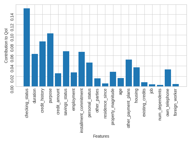
Finally, we can plot the mean contributions of each feature:
plt.style.use("seaborn-v0_8-whitegrid")

fig, ax = plt.subplots()
xai.plot.bar(unary_values.mean(), ax=ax)
ax.set_ylim(bottom=0)
ax.tick_params(labelrotation=90)
fig.tight_layout()
plt.show()
Total running time of the script: (1 minutes 28.645 seconds)